This section outlines the steps taken to clean and preprocess the U.S. exoneration dataset, with a specific focus on Illinois cases. The cleaning process organizes the raw data into a structured and usable format for exploratory data analysis (EDA) and subsequent analysis workflows. By the end of this phase, the dataset will be well-structured, free of inconsistencies, and ready for further exploratory data analysis and machine learning workflows.
Initial Overview of the Dataset
Loading the Dataset
The dataset is first loaded to inspect its structure and contents. The purpose of this step is to get an initial sense of the data types, potential missing values, and the distribution of key variables which helps inform the cleaning steps required to make the data consistent and analyzable.
Code
# Import necessary Libraries:import pandas as pd # Used for data management, exploration, and manipulationimport numpy as np # Used for numerical operations and array-based data processingimport seaborn as sns # Used for data visualization, especially for missing valuesimport matplotlib.pyplot as plt # Used for plotting and visualizing dataimport re # Used for handling and processing regular expressions, e.g., date cleaning# Load exoneration dataset:df = pd.read_csv('../../data/raw-data/US_exoneration_data.csv')print("Initial Dataset: ")pd.set_option('display.max_columns', None) # Enables display of every columndf.head()
Initial Dataset:
Last Name
First Name
Age
Race
Sex
State
County
Tags
Worst Crime Display
Sentence
Posting Date
OM Tags
F/MFE
FC
ILD
P/FA
DNA
MWID
OM
Date of Exoneration
Date of 1st Conviction
Date of Release
0
Abbitt
Joseph
31.0
Black
Male
North Carolina
Forsyth
CV;#IO;#SA
Child Sex Abuse
Life
9/1/11
NaN
NaN
NaN
NaN
NaN
DNA
MWID
NaN
9/2/09
6/22/95
9/2/09
1
Abbott
Cinque
19.0
Black
Male
Illinois
Cook
CIU;#IO;#NC;#P
Drug Possession or Sale
Probation
2/14/22
OF;#WH;#NW
NaN
NaN
NaN
P/FA
NaN
NaN
OM
2/1/22
3/25/08
3/25/08
2
Abdal
Warith Habib
43.0
Black
Male
New York
Erie
IO;#SA
Sexual Assault
20 to Life
8/29/11
OF;#WH;#NW;#WT
F/MFE
NaN
NaN
NaN
DNA
MWID
OM
9/1/99
6/6/83
9/1/99
3
Abernathy
Christopher
17.0
White
Male
Illinois
Cook
CIU;#CV;#H;#IO;#JV;#SA
Murder
Life without parole
2/13/15
OF;#WH;#NW;#INT
NaN
FC
NaN
P/FA
DNA
NaN
OM
2/11/15
1/15/87
2/11/15
4
Abney
Quentin
32.0
Black
Male
New York
New York
CV
Robbery
20 to Life
5/13/19
NaN
NaN
NaN
NaN
NaN
NaN
MWID
NaN
1/19/12
3/20/06
1/19/12
Subsetting the Data: Illinois
Before diving into the broader data cleaning process, I decided to narrow the scope of my research question to Illinois. This choice was intentional to focus the analysis on a specific region, ensuring that the findings are both relevant and manageable within the scope of this project. Illinois was selected because of its extensive record of exoneration cases, particularly in Cook Count (Chicago), which provides a valuable dataset for analyzing systemic issues within the criminal justice system. Chicago, in particular, has long been associated with significant racial disparities and deeply entrenched problems in policing and prosecution, making it a critical focal point for this analysis1. By focusing on Illinois, the dataset remains consistent in terms of jurisdictional laws and practices, allowing for a more accurate and concentrated exploration of patterns and trends in over-policing and wrongful convictions. This regional focus highlights the broader systemic failures of the criminal justice system while enabling a detailed examination of one of the most historically inequitable jurisdictions in terms of racial justice.
Filtering the Dataset
To isolate Illinois cases, the dataset was filtered by the state column, retaining only rows where the value matched “Illinois.” This step reduced the dataset to 548 rows, making it more manageable for analysis and visualization. Below is a preview of the filtered dataset:
Code
# Filter Data for Illinois: df = df[df['State'] =='Illinois']print("Number of exonerees for Illinois subset: " , df.shape[0]) df.head()
Number of exonerees for Illinois subset: 548
Last Name
First Name
Age
Race
Sex
State
County
Tags
Worst Crime Display
Sentence
Posting Date
OM Tags
F/MFE
FC
ILD
P/FA
DNA
MWID
OM
Date of Exoneration
Date of 1st Conviction
Date of Release
1
Abbott
Cinque
19.0
Black
Male
Illinois
Cook
CIU;#IO;#NC;#P
Drug Possession or Sale
Probation
2/14/22
OF;#WH;#NW
NaN
NaN
NaN
P/FA
NaN
NaN
OM
2/1/22
3/25/08
3/25/08
3
Abernathy
Christopher
17.0
White
Male
Illinois
Cook
CIU;#CV;#H;#IO;#JV;#SA
Murder
Life without parole
2/13/15
OF;#WH;#NW;#INT
NaN
FC
NaN
P/FA
DNA
NaN
OM
2/11/15
1/15/87
2/11/15
5
Abrego
Eruby
20.0
Hispanic
Male
Illinois
Cook
CDC;#H;#IO
Murder
90 years
8/25/22
OF;#WH;#NW;#WT;#INT;#PJ
NaN
FC
NaN
P/FA
NaN
MWID
OM
7/21/22
9/22/04
7/21/22
10
Adams
Demetris
22.0
Black
Male
Illinois
Cook
CIU;#IO;#NC;#P
Drug Possession or Sale
1 year
4/13/20
OF;#WH;#NW
NaN
NaN
NaN
P/FA
NaN
NaN
OM
2/11/20
9/8/04
12/26/04
15
Adams
Kenneth
22.0
Black
Male
Illinois
Cook
CDC;#H;#IO;#JI;#SA
Murder
75 years
8/29/11
PR;#OF;#WH;#NW;#KP;#WT
F/MFE
NaN
NaN
P/FA
DNA
MWID
OM
7/2/96
10/20/78
6/14/96
Handling Missing Data
Identifying Missing Data
Missing values are identified using isnull() to determine their extent and distribution across the dataset. The goal is to ensure that no critical data gaps remain unaddressed before proceeding with analysis.
Code
# Managing Missing Data - Identifying which columns have a lot of missing data:na_counts = df.isna().sum()print(na_counts)
Last Name                   0
First Name                  0
Age                         1
Race                        0
Sex                         0
State                       0
County                      0
Tags                       15
Worst Crime Display         0
Sentence                    0
Posting Date                0
OM Tags                    70
F/MFE                     474
FC                        410
ILD                       440
P/FA                       67
DNA                       482
MWID                      442
OM                         70
Date of Exoneration         0
Date of 1st Conviction      0
Date of Release             0
dtype: int64
Handling Missing Data
Rationale for Dropping Columns
The following columns were removed due to excessive missing data:
F/MFE, ILD, P/FA, DNA, MWID, FC: Each of these columns had more than 50% missing values, which made them unreliable for meaningful analysis. Removing them ensures the dataset remains robust and manageable without introducing bias from imputation.
Retaining “OM” and “OM Tags” Columns Initially, I removed the OM (Official Misconduct) and OM Tags columns, assuming their information would be captured in the general Tags column. However, during the exploratory data analysis (EDA), I discovered that these columns contained unique and valuable insights not present in the Tags column; as a result I retained them for further analysis.
Code
# Drop columns with excessive missing values: df_original = df.copy()df.drop(columns = ['F/MFE', 'ILD', 'P/FA', 'DNA', 'MWID', 'FC'], inplace =True)
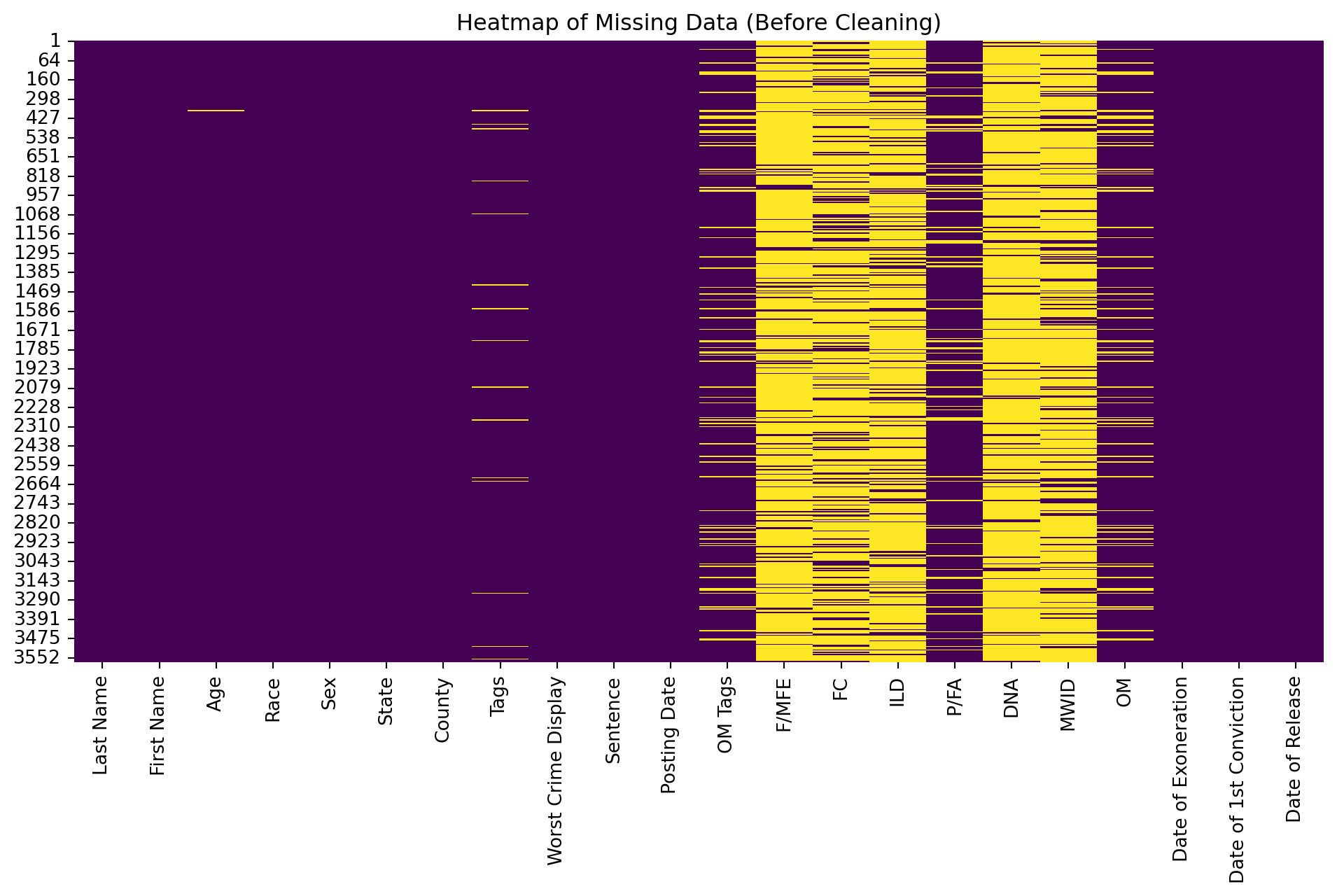
Visualizing Missing Data
To better understand the distribution of missing values, a heatmap is generated. This visualization provides a clear overview of where missing values occur, helping to decide which columns or rows to address in subsequent steps.
Heatmap of Missing Values (Before Cleaning)
A heatmap is generated to visualize the extent of missing data before cleaning. Columns with a high proportion of missing values are easily identifiable, providing a clear justification for their removal.
Code
# Heatmap of missing data before cleaning:plt.figure(figsize=(12, 6))sns.heatmap(df_original.isnull(), cbar=False, cmap='viridis')plt.title('Heatmap of Missing Data (Before Cleaning)')plt.show()
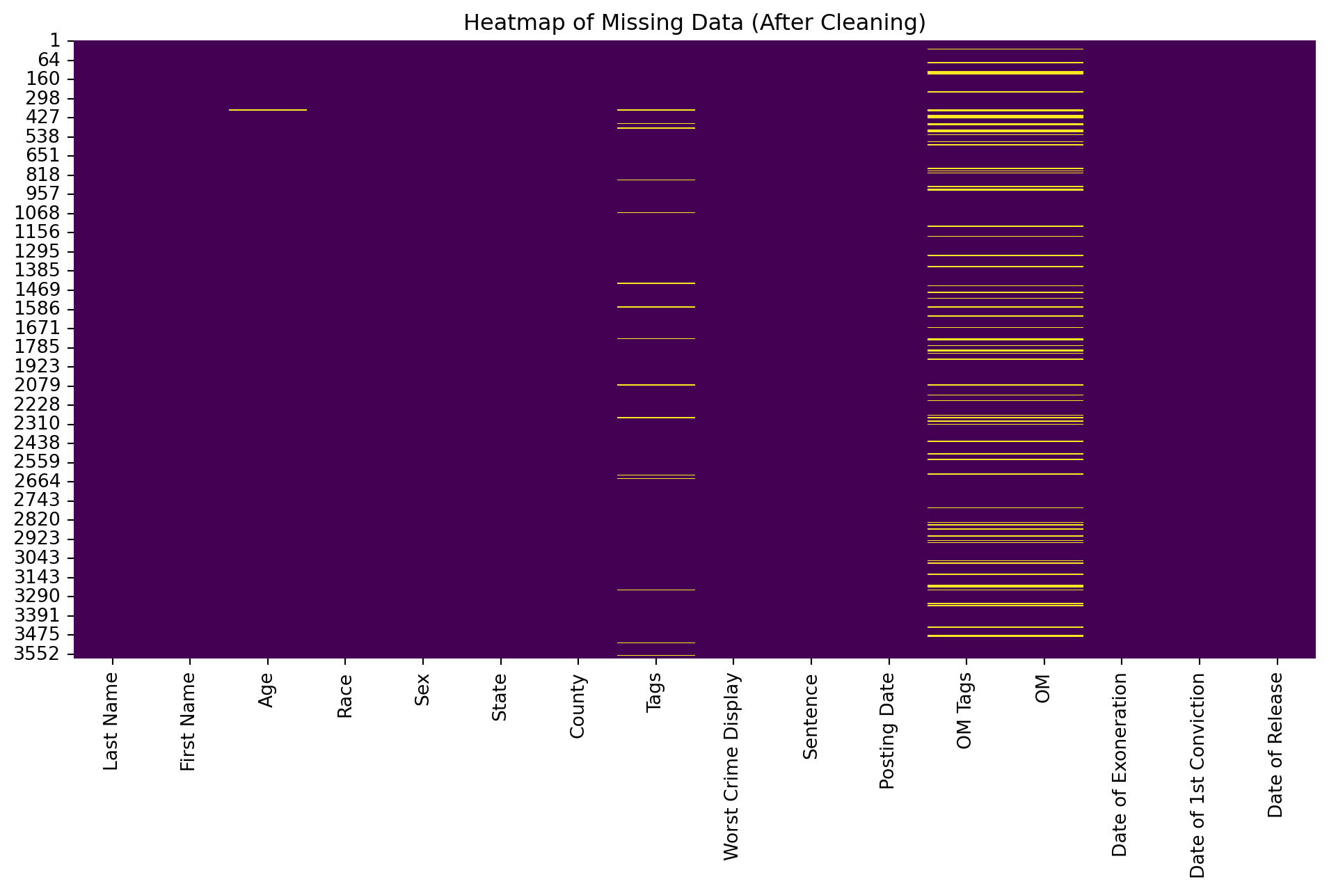
Heatmap of Missing Values (After Cleaning)
A second heatmap is generated after cleaning to confirm that all unnecessary columns with excessive missing values have been removed. This ensures the dataset is now complete and ready for further analysis.
Code
# Heatmap of missing data after cleaning:plt.figure(figsize=(12, 6))sns.heatmap(df.isnull(), cbar=False, cmap='viridis')plt.title('Heatmap of Missing Data (After Cleaning)')plt.show()
Column Standardization
To ensure consistency and simplify future operations, all column names were standardized by converting them to lowercase and replacing spaces with underscores (_). This transformation enhances readability, aligns with Python’s naming conventions, and makes column names easier to reference in code. For example, a column originally labeled First Name is now first_name.
Code
# Standardize column names by converting to lowercase and replacing spaces with '_':df.columns = df.columns.str.lower().str.replace(' ', '_')print(df.columns)
Additionally, the sex column was converted to lowercase to maintain uniformity across textual data. This step ensures that values like “Male” and “male” are treated equivalently during analysis, reducing potential discrepancies caused by case sensitivity.
Code
# Convert sex values to lowercase: df['sex'] = df['sex'].str.lower()df['sex'].head()
1     male
3     male
5     male
10    male
15    male
Name: sex, dtype: object
Data Type Correction and Formatting
Accurate data type formatting is essential for effective analysis. This section ensures that all variables are correctly identified as numerical, categorical, or date-time types so that they are ready for further processing.
Code
# Display data types for each column:print(df.dtypes)
last_name                  object
first_name                 object
age                       float64
race                       object
sex                        object
state                      object
county                     object
tags                       object
worst_crime_display        object
sentence                   object
posting_date               object
om_tags                    object
om                         object
date_of_exoneration        object
date_of_1st_conviction     object
date_of_release            object
dtype: object
Data Type Correction for Textual Data
Upon reviewing the data types, it was noted that several columns, such as Last Name, First Name, Race, State, County, and Worst Crime Display, were classified as object. While this is acceptable for textual data, converting these columns to string ensures consistency and prevents potential issues when performing text-specific operations. This transformation also allows for better optimization and clarity in the data processing pipeline. The changes were necessary to standardize the dataset and ensure compatibility with downstream analysis tasks.
last_name                 string[python]
first_name                string[python]
age                              float64
race                      string[python]
sex                       string[python]
state                     string[python]
county                    string[python]
tags                              object
worst_crime_display       string[python]
sentence                          object
posting_date                      object
om_tags                           object
om                                object
date_of_exoneration               object
date_of_1st_conviction            object
date_of_release                   object
dtype: object
Date-Time Conversion
All date columns (posting_date, date_of_exoneration, date_of_1st_conviction, date_of_release) are converted to datetime format. This transformation ensures consistency and allows for easier time-based calculations, such as measuring the time between conviction and exoneration.
Code
# Convert date columns into datetime format:for col in ['posting_date', 'date_of_exoneration', 'date_of_1st_conviction', 'date_of_release']:# Convert with explicit format (MM/DD/YY): df[col] = pd.to_datetime(df[col], format='%m/%d/%y', errors='coerce')print(df[['posting_date', 'date_of_exoneration', 'date_of_1st_conviction', 'date_of_release']].head())
last_name                 string[python]
first_name                string[python]
age                              float64
race                      string[python]
sex                       string[python]
state                     string[python]
county                    string[python]
tags                              object
worst_crime_display       string[python]
sentence                          object
posting_date              datetime64[ns]
om_tags                           object
om                                object
date_of_exoneration       datetime64[ns]
date_of_1st_conviction    datetime64[ns]
date_of_release           datetime64[ns]
dtype: object
Standardizing the sentence Column
The sentence column contains textual descriptions of sentencing outcomes, including terms like “Life without parole,” “Death,” or a specified number of years. To facilitate analysis, this column is transformed into a numerical format (sentence_in_years) by converting life sentences and probation to placeholder values and handling ranges or mixed units (e.g., years and months).
Code
# Print unique sentencing values for a better idea on how to best clean column: unique_sentences = df['sentence'].unique()print(unique_sentences)
['Probation' 'Life without parole' '90 years' '1 year' '75 years'
 '30 years' '55 years' '2 years' '3 years' '6 years' '45 years'
 '1 year and 6 months' '50 years' '60 years' 'Life' '80 years' '18 years'
 '4 years' '85 years' '20 years' '35 years' '2 years and 6 months'
 '82 years' '12 years' 'Not sentenced' '22 years' '32 years' 'Death'
 '5 years' '40 years' '25 years' '26 years' '4 years and 6 months'
 '9 years' '48 years' '30 days' '84 years' '3 months and 25 days'
 '2 years and 2 months' '3 months' '44 years' '6 months' '25 to 50 years'
 '29 years' '23 years' '31 years' '11 years' '8 years' '24 years'
 '3 years and four months' '42 years' '3 years and 6 months' '65 years'
 '76 years' '15 years' '50 to Life' '86 years' '70 years' '28 years'
 '13 years' '47 years' '36 years' '18 months' '1 year and 4 months'
 '8 years and 6 months' '6 years and 6 months' '58 years' '95 years'
 '7 years' '34 years' '62 years' '27 years' '69 years' '57 years'
 '50 to 100 years' '4 months' '4 years and 3 months' '37 years' '10 years'
 '67 years' '46 years' '17 years' '10 to 22 years' '6 years and 7 months'
 '5 years and 6 months' '2 Years']
Transforming the sentence Column
The sentence column is cleaned to convert textual descriptions into numerical values: 1. Probation and Not Sentenced are set to 0. 2. Life sentences and the death penalty are represented as 100 for placeholder analysis. 3. Ranges (e.g., “25 to 50 years”) are averaged to a single value. 4. Years and months are combined into total years for uniformity.
This standardization facilitates meaningful comparisons and quantitative analysis of sentencing patterns.
Code
def clean_sentence(value):""" Cleans the 'sentence' column values to numeric years for numerical EDA - Probation is represented as 0. - 'Not sentenced' is converted to np.nan. - 'Life' and 'Death' sentences are represented as 100 (placeholder). - Years and months are converted to a numeric value in years. """if value =='Probation':return0elif value =='Not sentenced':return np.nan # NaN for not sentencedelif'Life'in value or value =='Death':return100# Placeholder for life sentences or death penaltyelif'year'in value or'month'in value:# Handles ranges like '25 to 50 years'if'to'in value: years = [int(num) for num in re.findall(r'\d+', value)]returnsum(years) /len(years) # Average the range # Handle "X years and Y months"elif'and'in value: numbers = [float(num) for num in re.findall(r'\d+', value)]iflen(numbers) ==2: # Both years and months are present years, months = numbersreturn years + (months /12) # Convert months to yearseliflen(numbers) ==1: # Only one number is presentreturn numbers[0] # Treat it as years# Handle only months or only yearselif'months'in value: months =int(re.search(r'\d+', value).group())return months /12# Convert months to yearselse: # Only yearsreturnint(re.search(r'\d+', value).group())else:return np.nan # Anything unexpected as Nonedf['sentence_in_years'] = df['sentence'].apply(clean_sentence)# Check resultsdf[['sentence', 'sentence_in_years']].head(10)
sentence
sentence_in_years
1
Probation
0.0
3
Life without parole
100.0
5
90 years
90.0
10
1 year
1.0
15
75 years
75.0
21
Probation
0.0
22
Probation
0.0
24
30 years
30.0
25
55 years
55.0
45
1 year
1.0
Code
# Check updated data typesprint(df.dtypes)
last_name                 string[python]
first_name                string[python]
age                              float64
race                      string[python]
sex                       string[python]
state                     string[python]
county                    string[python]
tags                              object
worst_crime_display       string[python]
sentence                          object
posting_date              datetime64[ns]
om_tags                           object
om                                object
date_of_exoneration       datetime64[ns]
date_of_1st_conviction    datetime64[ns]
date_of_release           datetime64[ns]
sentence_in_years                float64
dtype: object
After transforming the sentence column into a numerical format, the new column, sentence_in_years is now represented as a float64, which aligns with the desired structure for numerical analysis. This conversion allows for quantitative exploration of the sentencing data, such as aggregations and comparisons, during later stages of analysis. The original sentence column is retained for reference purposes, as it preserves the detailed textual descriptions that might be useful for contextual insights. The tags, OM, and OM_tags columns will be addressed later, so for now the datatype may remain as an object.
Cleaning the tags and OM-tags Columns
The tags and OM-tags columns contain important categorical information about each exoneration case. To make this data more useful for analysis, both columns were transformed into multiple binary columns, where each tag indicates the presence (1) or absence (0) of a specific feature. Additionally, a tag_sum column was created to capture the total number of tags associated with each case, providing a summary metric.
The cleaning process involved the following steps:
Removing Unnecessary Characters:
Unwanted characters such as # were removed, and delimiters were standardized to ensure consistency in the data.
Splitting Tags:
The tags and OM-tags columns were split into individual values to facilitate binary encoding.
Renaming Binary Columns:
Each binary column was renamed using clear and descriptive labels by mapping the original tags to their definitions. This mapping process translated short tag codes into their full meanings, improving interpretability. For reference, the definitions of the tags are based on the descriptions provided by the National Registry of Exonerations2.
Adding a tag_sum Column:
A new column was created to calculate the total number of tags for each case, enabling easier analysis of case complexity.
This transformation ensures the data is well-structured and ready for exploratory analysis, providing detailed insights into the systemic patterns in exoneration cases.
Code
# Clean 'tags' column:df['tags'] = df['tags'].str.replace('#', '', regex=False).str.replace(";", ",")df['OM-tags'] = df['om_tags'].str.replace('#', '', regex=False).str.replace(";", ",")# Define the mapping for tags:tag_mapping = {"A": "arson","BM": "bitemark","CDC": "co_defendant_confessed","CIU": "conviction_integrity_unit","CSH": "child_sex_abuse_hysteria_case","CV": "child_victim","F": "female_exoneree","FED": "federal_case","H": "homicide","IO": "innocence_organization","JI": "jailhouse_informant","JV": "juvenile_defendant","M": "misdemeanor","NC": "no_crime_case","P": "guilty_plea_case","PH": "posthumous_exoneration","SA": "sexual_assault","SBS": "shaken_baby_syndrome_case","PR": "prosecutor_misconduct","OF": "police_officer_misconduct","FA": "forensic_analyst_misconduct","CW": "child_welfare_worker_misconduct","WH": "withheld_exculpatory_evidence","NW": "misconduct_that_is_not_withholding_evidence","KP": "knowingly_permitting_perjury","WT": "witness_tampering_or_misconduct_interrogating_co_defendant","INT": "misconduct_in_interrogation_of_exoneree","PJ": "perjury_by_official","PL": "prosecutor_lied_in_court"}# Split 'tags' and 'OM-tags' into lists:df['tags'] = df['tags'].apply(lambda x: x.split(',') ifisinstance(x, str) else x)df['OM-tags'] = df['OM-tags'].apply(lambda x: x.split(',') ifisinstance(x, str) else x)# Create binary columns for tags from both 'tags' and 'OM-tags':for tag in tag_mapping.keys():# Check if the tag exists in 'tags' or 'OM-tags': df[tag] = df.apply(lambda row: 1if (isinstance(row['tags'], list) and tag in row['tags']) or (isinstance(row['OM-tags'], list) and tag in row['OM-tags']) else0, axis=1 )# Rename the binary columns using the tag_mapping dictionary:df.rename(columns=tag_mapping, inplace=True)# Create `tag_sum` column to count the total number of tags for each exoneree:df['tag_sum'] = df[list(tag_mapping.values())].sum(axis=1)# Drop the original 'tags' and 'OM-tags' columns:df.drop(columns=['tags', 'om_tags', 'OM-tags'], inplace=True)df.head()
# Convert 'OM' column to binary (1 if "OM" is present, 0 otherwise)df['om'] = df['om'].apply(lambda x: 1ifstr(x).strip().upper() =="OM"else0)# Verify the transformationprint(df['om'].value_counts())
om
1    478
0     70
Name: count, dtype: int64
Merge with Geocoded Counties
The geocoded Illinois counties from Data Collection were merged into the main dataset:
Load and Standardize Data: Geocoded data was loaded, and column names were standardized to lowercase for consistency.
Filter Relevant Counties: The geocoded data was filtered to include only counties present in the main dataset.
Merge Data: Using a left join on county and state, geographic details (geocode_address, latitude, and longitude) were added to the dataset.
Code
# Read the geocoded population data from Data Collectiongeocode_unique = pd.read_csv("../../data/raw-data/geocoded_population_counties.csv")# Rename columns to lowercase for consistencygeocode_unique.rename(columns={"County": "county", "State": "state"}, inplace=True)# Filter geocode_unique to only include counties present in dfgeocode_unique_filtered = geocode_unique[ geocode_unique[['county', 'state']].apply(tuple, axis=1).isin(df[['county', 'state']].apply(tuple, axis=1))]# Merge the filtered geocoding data into dfdf = df.merge(geocode_unique_filtered, on=['county', 'state'], how='left')# Display the relevant columns to verify the mergeprint(df[['state', 'county', 'geocode_address', 'latitude', 'longitude']].head())
      state county                       geocode_address   latitude  longitude
0  Illinois   Cook  Cook County, Illinois, United States  41.819738 -87.756525
1  Illinois   Cook  Cook County, Illinois, United States  41.819738 -87.756525
2  Illinois   Cook  Cook County, Illinois, United States  41.819738 -87.756525
3  Illinois   Cook  Cook County, Illinois, United States  41.819738 -87.756525
4  Illinois   Cook  Cook County, Illinois, United States  41.819738 -87.756525
Calculating Years Lost
To quantify the years_lost due to wrongful conviction, this step calculates the difference in years between an individual’s date_of_1st_conviction and their date_of_release.
Code
# Calculate "years lost" as the difference in years between release and conviction:df['years_lost'] = (df['date_of_release'] - df['date_of_1st_conviction']).dt.days /365.25# Dividing by 365.25 accounts for leap years# Round the years lost to 2 decimal places:df['years_lost'] = df['years_lost'].round(2)# Updated DataFrame:print(df[['date_of_1st_conviction', 'date_of_release', 'years_lost']])
To improve readability and logical flow, the following changes were made to the column order:
Align Sentencing Data:
The sentence_in_years column was moved to appear immediately after sentence, ensuring that the cleaned numerical representation of sentencing data is logically aligned with its original textual description.
Reorganize Release and Years Lost:
The years_lost column was moved to appear immediately after date_of_release, facilitating easier comparison of release dates and the calculated time lost due to wrongful incarceration.
Group Geographic Data:
The latitude and longitude columns were moved to follow the county column, grouping geographic information together.
Code
# Reordering columns:columns =list(df.columns) #Aligning sentencing data: columns.insert(columns.index('sentence') +1, columns.pop(columns.index('sentence_in_years'))) # Move 'sentence_in_years'#Reorganizing release and years lostcolumns.insert(columns.index('date_of_release') +1, columns.pop(columns.index('years_lost'))) #Move 'years_lost' # Move 'latitude' and 'longitude' after 'county'columns.insert(columns.index('county') +1, columns.pop(columns.index('latitude')))columns.insert(columns.index('county') +2, columns.pop(columns.index('longitude')))df = df[columns] # Reorder DataFramedf.head(10)
The final cleaned dataset is saved as illinois_exoneration_data.csv, ensuring that all preprocessing steps are reproducible, and the dataset can be used consistently across various analysis stages.
Code
df.to_csv('../../data/processed-data/illinois_exoneration_data.csv', index=False)print("Data saved to 'illinois_exoneration_data.csv'")
Data saved to 'illinois_exoneration_data.csv'
Illinois Arrest Data Cleaning
Introduction and Motivation
This section documents the steps taken to clean and preprocess the Illinois arrest dataset. Similarly to the U.S. exoneration dataset, the goal is to transform the raw data into a structured and reliable format for analysis. However, this dataset required fewer cleaning steps due to its uniform structure and consistent formatting.
By the end of this phase, the Illinois arrest dataset will be well-prepared for exploratory data analysis (EDA) and integration into broader investigative workflows.
Initial Overview of the Dataset
The dataset is first loaded to inspect its structure and contents.
Code
# Load exoneration dataset:arrest_data = pd.read_csv('../../data/raw-data/illinois_arrest_explorer_data.csv')print("Initial Dataset: ")pd.set_option('display.max_columns', None) # Enables display of every columnarrest_data.head()
Initial Dataset:
Year
race
county_Adams
county_Alexander
county_Bond
county_Boone
county_Brown
county_Bureau
county_Calhoun
county_Carroll
county_Cass
county_Champaign
county_Christian
county_Clark
county_Clay
county_Clinton
county_Coles
county_Cook Chicago
county_Cook County Suburbs
county_Crawford
county_Cumberland
county_Dekalb
county_Dewitt
county_Douglas
county_Dupage
county_Edgar
county_Edwards
county_Effingham
county_Fayette
county_Ford
county_Franklin
county_Fulton
county_Gallatin
county_Greene
county_Grundy
county_Hamilton
county_Hancock
county_Hardin
county_Henderson
county_Henry
county_Iroquois
county_Jackson
county_Jasper
county_Jefferson
county_Jersey
county_Jo Daviess
county_Johnson
county_Kane
county_Kankakee
county_Kendall
county_Knox
county_Lake
county_Lasalle
county_Lawrence
county_Lee
county_Livingston
county_Logan
county_Macon
county_Macoupin
county_Madison
county_Marion
county_Marshall
county_Mason
county_Massac
county_Mcdonough
county_Mchenry
county_Mclean
county_Menard
county_Mercer
county_Monroe
county_Montgomery
county_Morgan
county_Moultrie
county_Non County Agencies
county_Ogle
county_Peoria
county_Perry
county_Piatt
county_Pike
county_Pope
county_Pulaski
county_Putnam
county_Randolph
county_Richland
county_Rock Island
county_Saline
county_Sangamon
county_Schuyler
county_Scott
county_Shelby
county_St. Clair
county_Stark
county_Stephenson
county_Tazewell
county_Union
county_Vermilion
county_Wabash
county_Warren
county_Washington
county_Wayne
county_White
county_Whiteside
county_Will
county_Williamson
county_Winnebago
county_Woodford
0
2001
African American
226
147
25
18
18
48
6
12
1
2059
16
6
1
22
130
86781
26301
6
1
342
11
18
2265
1
1
108
6
1
6
25
1
1
52
1
1
1
6
92
250
580
1
246
6
16
16
2804
1669
122
314
5712
184
6
86
180
71
1104
34
1567
146
6
1
91
105
213
905
1
6
20
38
287
6
1
57
3403
60
1
13
1
153
1
81
6
1215
104
2200
6
1
1
2462
1
355
168
17
876
6
46
25
6
16
128
3000
75
2509
42
1
2001
Asian
1
1
1
1
1
1
1
1
1
49
1
1
1
1
1
722
460
1
1
15
1
1
139
1
1
1
1
1
1
1
1
1
1
1
1
1
1
1
1
1
1
1
1
1
1
97
1
1
1
135
1
1
1
1
1
1
1
12
1
1
1
1
6
6
16
1
1
1
1
1
1
1
1
12
1
1
1
1
1
1
1
1
1
1
17
1
1
1
6
1
1
6
1
1
1
1
1
1
1
1
14
1
28
1
2
2001
Hispanic
1
1
1
1
1
1
1
1
1
1
1
1
1
1
1
1
1
1
1
1
1
1
1
1
1
1
1
1
1
1
1
1
1
1
1
1
1
1
1
1
1
1
1
1
1
1
1
1
1
1
1
1
1
1
1
1
1
1
1
1
1
1
1
1
1
1
1
1
1
1
1
1
1
1
1
1
1
1
1
1
1
1
1
1
1
1
1
1
1
1
1
1
1
1
1
1
1
1
1
1
1
1
1
1
3
2001
Native American
1
1
1
1
1
1
1
1
1
1
1
1
1
1
1
146
30
1
1
1
1
1
17
1
1
1
1
1
1
1
1
1
1
1
1
1
1
1
1
1
1
1
1
1
1
16
1
1
1
10
1
1
1
1
1
1
1
6
1
1
1
1
1
1
6
1
1
1
1
1
1
1
1
1
1
1
1
1
1
1
1
1
1
1
6
1
1
1
1
1
1
1
1
1
1
1
1
1
1
1
1
1
6
1
4
2001
White
939
52
209
674
107
509
139
298
88
2334
335
264
117
229
1635
37099
36690
470
164
1740
539
181
13019
301
41
986
382
217
724
926
19
57
1014
78
206
75
134
569
585
857
87
607
575
532
198
9634
1607
1465
1160
15136
2689
412
845
1146
586
1388
523
4359
571
263
274
455
1007
3879
2285
92
410
572
749
1053
149
1
1009
3120
430
211
368
45
248
151
460
323
3117
711
3635
274
22
486
1601
59
644
1804
327
1743
324
444
265
245
668
1304
4144
631
4253
462
Column Renaming and Consolidation
To streamline the Illinois arrest dataset and improve clarity, the following transformations were applied:
Removing Prefixes for Simplicity:
Columns with the county_ prefix were renamed by removing the prefix and capitalizing the remaining column names. This makes the column headers cleaner and more intuitive for analysis.
Standardizing Race Terminology:
The term “African American” in the race column was replaced with “Black” to ensure consistency with the exoneration dataset.
Consolidating Cook County Data:
The columns Cook Chicago and Cook County Suburbs were combined into a single Cook column. This consolidation simplifies the data and groups all arrest information related to Cook County into a unified metric.
Code
# Rename columns by removing 'county_' prefix:arrest_data.columns = [col.replace('county_', '').capitalize() if col.startswith('county_') else col for col in arrest_data.columns]# Rename "African American" to "Black" in the column names:arrest_data['race'] = arrest_data['race'].replace('African American', 'Black')# Combine "Cook Chicago" and "Cook County Suburbs" into a single "Cook" column:arrest_data['Cook'] = arrest_data['Cook chicago'] + arrest_data['Cook county suburbs']# Drop the old columns:arrest_data.drop(columns=['Cook chicago', 'Cook county suburbs'], inplace=True)arrest_data.head(1)
Year
race
Adams
Alexander
Bond
Boone
Brown
Bureau
Calhoun
Carroll
Cass
Champaign
Christian
Clark
Clay
Clinton
Coles
Crawford
Cumberland
Dekalb
Dewitt
Douglas
Dupage
Edgar
Edwards
Effingham
Fayette
Ford
Franklin
Fulton
Gallatin
Greene
Grundy
Hamilton
Hancock
Hardin
Henderson
Henry
Iroquois
Jackson
Jasper
Jefferson
Jersey
Jo daviess
Johnson
Kane
Kankakee
Kendall
Knox
Lake
Lasalle
Lawrence
Lee
Livingston
Logan
Macon
Macoupin
Madison
Marion
Marshall
Mason
Massac
Mcdonough
Mchenry
Mclean
Menard
Mercer
Monroe
Montgomery
Morgan
Moultrie
Non county agencies
Ogle
Peoria
Perry
Piatt
Pike
Pope
Pulaski
Putnam
Randolph
Richland
Rock island
Saline
Sangamon
Schuyler
Scott
Shelby
St. clair
Stark
Stephenson
Tazewell
Union
Vermilion
Wabash
Warren
Washington
Wayne
White
Whiteside
Will
Williamson
Winnebago
Woodford
Cook
0
2001
Black
226
147
25
18
18
48
6
12
1
2059
16
6
1
22
130
6
1
342
11
18
2265
1
1
108
6
1
6
25
1
1
52
1
1
1
6
92
250
580
1
246
6
16
16
2804
1669
122
314
5712
184
6
86
180
71
1104
34
1567
146
6
1
91
105
213
905
1
6
20
38
287
6
1
57
3403
60
1
13
1
153
1
81
6
1215
104
2200
6
1
1
2462
1
355
168
17
876
6
46
25
6
16
128
3000
75
2509
42
113082
Handling Placeholder Values
During preprocessing, it was observed that the dataset contains 1s in certain fields. To address this all 1s in the dataset were replaced with 0s to ensure the integrity of the analysis. This decision ensures that the data is not skewed by suspicious or placeholder values, which could misrepresent trends or introduce bias into the results.
Note: The reasoning behind the presence of these placeholder values is discussed further in the Data Collection section.
Code
# Replace 1s with 0s: arrest_data.replace(1, 0, inplace=True)# Display the updated dataset to confirm changes:arrest_data.head()arrest_data.head()
Year
race
Adams
Alexander
Bond
Boone
Brown
Bureau
Calhoun
Carroll
Cass
Champaign
Christian
Clark
Clay
Clinton
Coles
Crawford
Cumberland
Dekalb
Dewitt
Douglas
Dupage
Edgar
Edwards
Effingham
Fayette
Ford
Franklin
Fulton
Gallatin
Greene
Grundy
Hamilton
Hancock
Hardin
Henderson
Henry
Iroquois
Jackson
Jasper
Jefferson
Jersey
Jo daviess
Johnson
Kane
Kankakee
Kendall
Knox
Lake
Lasalle
Lawrence
Lee
Livingston
Logan
Macon
Macoupin
Madison
Marion
Marshall
Mason
Massac
Mcdonough
Mchenry
Mclean
Menard
Mercer
Monroe
Montgomery
Morgan
Moultrie
Non county agencies
Ogle
Peoria
Perry
Piatt
Pike
Pope
Pulaski
Putnam
Randolph
Richland
Rock island
Saline
Sangamon
Schuyler
Scott
Shelby
St. clair
Stark
Stephenson
Tazewell
Union
Vermilion
Wabash
Warren
Washington
Wayne
White
Whiteside
Will
Williamson
Winnebago
Woodford
Cook
0
2001
Black
226
147
25
18
18
48
6
12
0
2059
16
6
0
22
130
6
0
342
11
18
2265
0
0
108
6
0
6
25
0
0
52
0
0
0
6
92
250
580
0
246
6
16
16
2804
1669
122
314
5712
184
6
86
180
71
1104
34
1567
146
6
0
91
105
213
905
0
6
20
38
287
6
0
57
3403
60
0
13
0
153
0
81
6
1215
104
2200
6
0
0
2462
0
355
168
17
876
6
46
25
6
16
128
3000
75
2509
42
113082
1
2001
Asian
0
0
0
0
0
0
0
0
0
49
0
0
0
0
0
0
0
15
0
0
139
0
0
0
0
0
0
0
0
0
0
0
0
0
0
0
0
0
0
0
0
0
0
97
0
0
0
135
0
0
0
0
0
0
0
12
0
0
0
0
6
6
16
0
0
0
0
0
0
0
0
12
0
0
0
0
0
0
0
0
0
0
17
0
0
0
6
0
0
6
0
0
0
0
0
0
0
0
14
0
28
0
1182
2
2001
Hispanic
0
0
0
0
0
0
0
0
0
0
0
0
0
0
0
0
0
0
0
0
0
0
0
0
0
0
0
0
0
0
0
0
0
0
0
0
0
0
0
0
0
0
0
0
0
0
0
0
0
0
0
0
0
0
0
0
0
0
0
0
0
0
0
0
0
0
0
0
0
0
0
0
0
0
0
0
0
0
0
0
0
0
0
0
0
0
0
0
0
0
0
0
0
0
0
0
0
0
0
0
0
0
2
3
2001
Native American
0
0
0
0
0
0
0
0
0
0
0
0
0
0
0
0
0
0
0
0
17
0
0
0
0
0
0
0
0
0
0
0
0
0
0
0
0
0
0
0
0
0
0
16
0
0
0
10
0
0
0
0
0
0
0
6
0
0
0
0
0
0
6
0
0
0
0
0
0
0
0
0
0
0
0
0
0
0
0
0
0
0
6
0
0
0
0
0
0
0
0
0
0
0
0
0
0
0
0
0
6
0
176
4
2001
White
939
52
209
674
107
509
139
298
88
2334
335
264
117
229
1635
470
164
1740
539
181
13019
301
41
986
382
217
724
926
19
57
1014
78
206
75
134
569
585
857
87
607
575
532
198
9634
1607
1465
1160
15136
2689
412
845
1146
586
1388
523
4359
571
263
274
455
1007
3879
2285
92
410
572
749
1053
149
0
1009
3120
430
211
368
45
248
151
460
323
3117
711
3635
274
22
486
1601
59
644
1804
327
1743
324
444
265
245
668
1304
4144
631
4253
462
73789
Exporting Cleaned and Aggregated Datasets
1. Exporting the Cleaned Dataset
After cleaning the Illinois arrest dataset, the cleaned version was saved as a CSV file. This dataset retains the original structure, including arrest counts broken down by race, county, and year. Maintaining the year-specific information allows for detailed time-series analysis and year-over-year comparisons.
Code
arrest_data.to_csv('../../data/processed-data/arrest_data_by_year.csv', index=False)print("Data saved to 'arrest_data_by_year.csv'")
Data saved to 'arrest_data_by_year.csv'
2. Aggregating Arrest Data by Race and County
The arrest data was aggregated to simplify the analysis by summing totals across all years for each race and county. This step removes the Year column and groups arrests solely by race and county.
Steps:
- Grouped the dataset by the race column.
- Summed arrest counts for each county across all years.
- Reset the index for a clean, tabular structure.
Code
# Aggregate totals across years for each race:aggregated_data = arrest_data.groupby('race').sum(numeric_only=True)aggregated_data = aggregated_data.drop(columns=['Year'])aggregated_data = aggregated_data.reset_index()# Preview the aggregated data:aggregated_data.head()
race
Adams
Alexander
Bond
Boone
Brown
Bureau
Calhoun
Carroll
Cass
Champaign
Christian
Clark
Clay
Clinton
Coles
Crawford
Cumberland
Dekalb
Dewitt
Douglas
Dupage
Edgar
Edwards
Effingham
Fayette
Ford
Franklin
Fulton
Gallatin
Greene
Grundy
Hamilton
Hancock
Hardin
Henderson
Henry
Iroquois
Jackson
Jasper
Jefferson
Jersey
Jo daviess
Johnson
Kane
Kankakee
Kendall
Knox
Lake
Lasalle
Lawrence
Lee
Livingston
Logan
Macon
Macoupin
Madison
Marion
Marshall
Mason
Massac
Mcdonough
Mchenry
Mclean
Menard
Mercer
Monroe
Montgomery
Morgan
Moultrie
Non county agencies
Ogle
Peoria
Perry
Piatt
Pike
Pope
Pulaski
Putnam
Randolph
Richland
Rock island
Saline
Sangamon
Schuyler
Scott
Shelby
St. clair
Stark
Stephenson
Tazewell
Union
Vermilion
Wabash
Warren
Washington
Wayne
White
Whiteside
Will
Williamson
Winnebago
Woodford
Cook
0
Asian
12
0
0
22
0
0
0
0
0
1186
0
0
0
6
0
0
0
301
0
0
4509
6
0
51
6
0
12
0
0
0
12
0
0
0
0
12
0
166
0
12
0
0
0
2239
30
66
0
2562
164
0
0
81
18
76
0
550
0
0
0
45
66
498
564
0
0
0
18
12
0
0
6
381
6
0
0
0
12
0
0
0
250
0
500
0
0
0
382
0
12
126
0
0
0
42
0
0
0
30
1443
36
767
46
26764
1
Black
4022
2722
533
2410
92
780
18
292
235
45547
459
187
75
877
4029
280
117
16146
594
499
59262
119
6
3293
588
275
520
627
6
110
2249
0
122
0
207
2131
3283
13120
45
5960
526
943
281
59806
27437
4308
7545
78841
7344
337
1654
4521
2353
27094
818
51485
4542
123
218
1731
4214
6581
27867
189
268
885
1275
7157
165
693
1685
79960
1901
358
519
18
3384
42
1731
213
26048
1795
63703
81
0
110
60744
24
11866
8363
399
17641
153
1024
489
91
464
2893
58968
4809
55837
2841
1772659
2
Hispanic
6
0
6
516
0
114
0
34
68
983
0
6
0
91
120
18
18
1783
84
147
13828
0
0
51
35
67
22
0
0
30
470
0
6
0
11
18
104
186
0
160
24
101
0
14151
634
264
323
10219
762
0
136
417
49
113
0
333
25
12
10
0
138
4126
1439
0
0
16
12
124
0
0
350
0
43
0
18
0
104
0
79
18
1135
0
29
12
0
0
449
0
39
192
18
0
0
142
12
0
6
436
3822
217
3522
63
144574
3
Native American
0
0
0
0
0
0
0
0
0
297
0
0
0
0
0
0
0
30
0
0
703
0
0
0
0
0
0
6
0
0
0
0
0
0
0
0
0
0
0
0
0
0
0
149
0
12
0
220
6
0
0
0
0
6
0
65
0
0
0
0
0
18
24
0
0
0
0
0
0
0
0
42
0
0
0
0
0
0
0
0
0
0
29
0
0
6
42
0
6
6
0
0
0
0
0
0
0
0
108
0
147
0
2351
4
White
16743
1340
3964
16580
1812
9593
1844
5530
2826
41996
10983
6714
4818
8858
23779
8663
4228
35622
7121
5676
215397
7031
1019
23978
9115
4630
22754
14545
838
5147
18813
1218
5203
1766
2653
11472
11041
16698
3124
14526
14337
7841
3325
170618
31714
27222
20553
188224
54179
8499
13856
20172
14366
30283
12071
130786
19686
4240
6970
8491
18618
101548
48554
3974
7257
10734
16631
23129
2920
751
19240
64589
12123
4323
7890
795
4457
1683
12061
6823
53728
12729
82714
2136
585
8671
49390
1442
13615
61546
6165
30772
6491
7459
5220
5146
11318
22690
97863
26871
85292
12676
1174775
Code
aggregated_data.to_csv('../../data/processed-data/aggregated_arrests_2001_to_2021.csv', index=False)print("Data saved to 'aggregated_arrests_2001_to_2021.csv'")
Data saved to 'aggregated_arrests_2001_to_2021.csv'
Mass Incarceration Racial Geography Data Cleaning
Introduction and Motivation
This section documents the minimal cleaning performed on the racial geography dataset which provides population and incarceration statistics by race, making it an essential input for balancing counterfactual data for supervised learning.
Unlike other datasets, this required minimal preprocessing due to its clean structure and consistent formatting. The primary cleaning steps involved standardizing column names for uniformity.
By the end of this step, the dataset is ready for use in data balancing and then machine learning.
Initial Overview of the Dataset
The dataset is first loaded to inspect its structure and contents.
Ratio of Overrepresentation of Whites Incarcerated Compared to Whites Non-Incarcerated
Ratio of Overrepresentation of Blacks Incarcerated Compared to Blacks Non-Incarcerated
Ratio of Overrepresentation of Latinos Incarcerated Compared to Latinos Non-Incarcerated
0
Adams County
Illinois
67103
62414
2331
776
110
73
36
0
66993
62341
2295
776
0.71
9.54
0.00
1
Alexander County
Illinois
8238
4983
2915
155
411
89
242
79
7827
4894
2673
76
0.35
1.72
19.82
2
Bond County
Illinois
17768
15797
1080
547
1542
500
657
304
16226
15297
423
243
0.34
16.32
13.14
3
Boone County
Illinois
54165
40757
1064
10967
71
38
12
21
54094
40719
1052
10946
0.71
8.71
1.46
4
Brown County
Illinois
6937
5191
1280
402
2059
419
1267
367
4878
4772
13
35
0.21
227.91
24.76
Standardizing Column Names
To improve readability and simplifyfurther processing, the column names in the dataset were converted to lowercase and spaces were replaced with underscores.
Code
representation_df.columns = representation_df.columns.str.lower().str.replace(' ', '_')representation_df.head()# Remove county from county name representation_df['county'] = representation_df['county'].str.replace(' County', '', regex=False)representation_df.head()
The final cleaned dataset is saved as representation_by_county.csv.
Code
representation_df.to_csv('../../data/processed-data/representation_by_county.csv', index=False)print("Data saved to 'representation_by_county_raw.csv'")
2. University of California Irvine Newkirk Center for Science & Society, & Michigan State University College of Law, U. of M. L. S. (2024). Exoneration DetailList. In The National Registry of Exonerations. https://www.law.umich.edu/special/exoneration/Pages/detaillist.aspx